Chapter 4 Passive Membrane Models

4.1 Vocabulary

Depolarization
Voltage threshold
Positive Feedback
Hyperpolarization
Negative Feedback
Membrane Potential
Sodium-Potassium Pump
Nernst potential / Reversal potential
Equilibrium Potential
Driving Force
Conductance
Capacitor
Leak Current
Leaky Integrate and Fire Model

4.2 Introduction

4.3 Membrane potentials and electrochemical gradients

Before going into ways of modeling action potentials, let’s further explore what an action potential is. Within a neuron, there resides a higher concentration of positively charged potassium ions, whereas outside of a neuron, there resides a higher concentration of positively charged sodium ions. However, there is an electrical and concentration difference between the intracellular and extracellular regions of the cell. The electrical difference, which occurs due to the difference in charge of different ions across the cell membrane, and the concentration difference, which is governed by the distribution of ions across the cell membrane, keep the cell in balance. Due to the higher concentration of sodium ions outside the cell, as well as their positive charge, the extracellular area is positive. Then, due the higher concentration of potassium ions inside the cell (which has an equilibrium potential of -90mV) as well as other negatively charged intracellular molecules, and a higher concentration of sodium outside the cell (which has an equilibrium potential of +55mV), the inside of a cell has a a more net negative charge relative to the outside. This feature illustrates the cause of the negative resting potential of a neuron.

There are two types of ion channels that continually contribute to the equilibrium between the cell’s electrical and concentration gradients. These channels are leakage channels and the sodium-potassium pump, which reside on the cell’s membrane. The sodium-potassium pump requires an input of one ATP to export three intracellular sodium ions and import two extracellular potassium ions against their electrical and concentration gradients. This pump takes energy because it is actively pushing ions against where they want to go. In addition to this, the leakage channels allow for ions to constantly move passively in and out of the cell with the flow of their opposing electrical and concentration gradients.

4.4 Phases of the action potential

4.4.1 Positive feedback and depolarization

Stimulation to the neuron will cause a positive increase in the intracellular voltage, due to the influx of sodium ions, beyond its voltage threshold. This positive increase across the threshold initiates the activation of both the voltage-gated sodium and voltage-gated potassium channels. The term voltage-gated indicates that these channels will either open or close when a specified intracellular voltage is reached. However, an important distinction between the two channels is that the voltage-gated sodium channels open much faster than the potassium channels. Thus, the quick reaction of the sodium channels causes an influx of intracellular sodium ions as they flow through the open voltage-gated sodium channels, causing the cell’s membrane potential to become more net positive. This process of positive ions flowing into the cell can be referred to as the rising phase, or depolarization. When depolarization happens, it causes additional sodium channels to open, which causes further depolarization. This phenomenon is called positive feedback. Positive feedback can be defined as a deviation reinforced by an action in the same direction, thus emphasizing that deviation. This positive feedback begins if the voltage threshold is met, and the loop of depolarization is a process that perpetuates itself.

Figure 4.1: An illustration of the positive feedback loop that perpetuates the depolarization of a cell.

4.4.2 Negative feedback and repolarization

The membrane potential will begin to approach the equilibrium potential for sodium due to a higher membrane permeability of this ion during depolarization. Before the membrane potential reaches the equilibrium potential of sodium, this triggers the inactivation of voltage-gated sodium channels, thus ending the positive feedback loop. This prevents the further exchange of sodium ions along their electrical and concentration gradient into the cell. Additionally, slow-reacting voltage-gated potassium channels activate and lead to the net flow of positively charged potassium ions along their electrical concentration gradient out of the cell. This action is characterized by the peak of an action potential, which then leads into the falling phase, or repolarization. Repolarization is the process of positive potassium ions flowing out of the cell, thus causing the membrane potential to decrease. The process of repolarization back to the cell’s initial resting potential is reinforced by a process called negative feedback. Negative feedback can be defined as a deviation offset by action in the opposite direction, thus re-establishing the “normal state.” This repolarization due to negative feedback eventually returns the cell’s voltage back to its resting potential.

Figure 4.2: An illustration of the negative feedback loop that hat re-establishes the normal resting potential of the cell membrane.

However, due to the potassium channels being slow, they are also slow to close once the cell has reached its initial resting potential. This means that even when the cell is appropriately negative, there are still potassium ions flowing out. This causes the voltage to fall slightly below the resting potential, a feature which we call the undershoot or hyperpolarization. The continuous function of sodium-potassium pumps and the leakage channels ultimately compensate for this slight undershoot, and re-establishes the initial resting potential.

To recap, the positive feedback causes a spike in membrane potential and the negative feedback stabilizes.

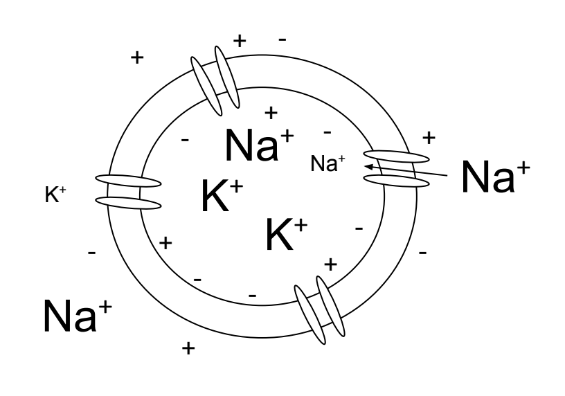
A cell at rest has more potassium ions intracellular than extracellular and more sodium ions extracellular than intracellular. There is a negative net charge within the cell being maintained by the voltage gradient.

Figure 4.3: A cell at rest has more potassium ions intracellular than extracellular and more sodium ions extracellular than intracellular. There is a negative net charge within the cell being maintained by the voltage gradient.

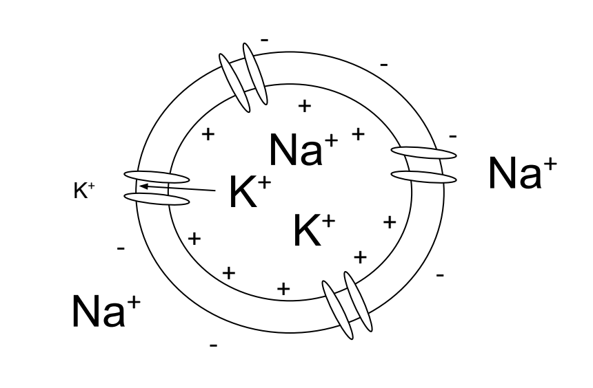
Figure 4.4: When the cell becomes depolarized sodium ions enter the cell. The charge within the cell becomes more positive.

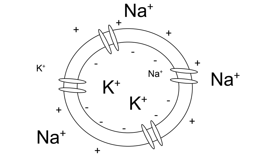
When the cell repolarizes potassium ions leave the cell. The charge within the cell go from positive to negative as it goes back to the resting state.

Figure 4.5: When the cell repolarizes potassium ions leave the cell. The charge within the cell go from positive to negative as it goes back to the resting state.

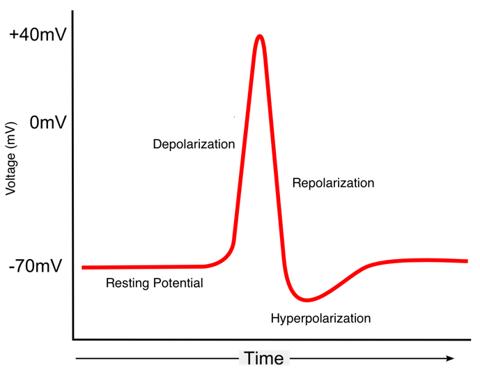
Figure 4.6: Example of an action potential.

4.5 Nernst equilibrium potential

The electrical potential generated in a neuron is the result of ions flowing across the neuron’s membrane which is caused by the following two principles: opposite charges attract, and concentration gradients seek to equalize. This electrical potential, generated by the sum of all electrical concentration gradients of each species of intracellular and extracellular ions at a specified time, is referred to as the membrane potential. In order for ions to flow, a concentration gradient must be established because the difference in ion distribution across the membrane leads the ions to either pass into or out of the neuron in an attempt to equalize. Thus, in order to build up a charge, we must create an unequal distribution of ions across the membrane relative to one another. This is accomplished by the sodium-potassium pump. This pump, which is suggested to use roughly 50% of total brain energy, pumps three sodium ions out of the neuron for every two potassium ions pumped in, thus forming the two respective concentration gradients [1].

With the concentration gradient established, the sodium and potassium ions will flow down the concentration gradients when their respective channels open, generating an electrical current that propagates down the axon. However, we must also take into account the fact that each ion possesses a charge–or charges in the case of Ca++ and Mg++–and that as this charge builds up on one side of the cell, generating an electrical force that will begin to repel ions with similar charge as they try to flow down their concentration gradient. This forms the electrical gradient, which along with the concentration gradient, dictates ion movement and the membrane potential. When the force of the concentration gradient matches the electrical force attracting or repelling the ion, it is known as the Nernst potential, which may also be referred to as the reversal potential. Each species of ion (i.e. sodium and potassium respectively) possess its own Nernst potential. Thus, the sum of Nernst potentials at a specified time can be summed in order to accurately predict the membrane potential at that time. Nernst potentials are especially important because they allow us to calculate the membrane voltage when a particular ion is in equilibrium, which helps to define the role it plays in an action potential.

The Nernst potential for an ion can be derived from the following equation: \[E_{ion} = \frac{RT}{zF}ln(\frac{[out]}{[in]}) \]

Expression	Meaning
\(E_{ion}\)	Nernst potential
R	Gas constant: 8.314 \(J/mol \cdot K\)
ln()	Natural log
z	Valence
T	Temperature in Kelvin
F	Faraday constant: 96485.3 C/mol
[out]	Extracellular ion concentration
[in]	Intracellular ion concentration

While the Nernst potential will give the equilibrium point for a single ion, it also has a relation to the equilibrium potential or the resting potential the membrane, which is potential at which there is no net flow of ions, leading to a halt in the flow of electric current. The equilibrium potential is really a weighted average of all of the Nernst potentials and is modeled by the Goldman-Hodgkin-Katz equation which is shown below: \[V_{m} = \frac{RT}{F}ln(\frac{P_{K}[K+]_{out}+P_{Na}[Na+]_{out}+P_{Cl}[Cl-]_{in}}{P_{K}[K+]_{in}+P_{Na}[Na+]_{in}+P_{Cl}[Cl-]_{out}}) \]

This equation utilizes the membrane permeability, P, in conjunction with the concentration of each ion inside and outside of the cell to produce the equilibrium potential of a membrane. Using this equation alongside the Nernst potential, the driving force, which is a representation of the pressure for an ion to move in or out of the cell, can be calculated using the following equation: \[DF = V_{m}-E_{ion} \]

The Nernst Potential, the Goldman-Hodgkin-Katz equation, and the driving force present necessary calculations that allow for better understanding of the flow of ions in relation to an action potential.

Worked Example:
Consider the following table of ion concentrations and relative permeabilities:

Ion	Intracellular concentration (mM)	Extracellular concentration (mM)	Permeability
K+	150	4	1
Na+	15	145	0.05
Cl-	10	110	0.45

If the extracellular concentration of Na+ was increased by a factor of ten:
a. What is the new Nernst potential for sodium?
b. What is the resting potential of the neuron?

Solution, part a
The Nernst equation is: \(E_{ion} = \frac{RT}{zF}ln\frac{[ion]_{outside}}{[ion]_{inside}}\) in which:

R is the ideal gas constant: 8.314 \(kg \cdot m^2 \cdot K^{1} \cdot mol^{-1}s^{-2}\)
T is the temperature in Kelvin: (310 K at human temperature)
z is the valence. Here, we use +1 because the Na+ ion has a charge of +1.
F is Faraday’s constant: 96.49 \(kJ \cdot V^{-1} \cdot mol^{-1}\)
Extracellular sodium is increased by a factor of 10: \([Na+]_{outside}\) = 10 * 145 mM = 1450 mM.

From these values:
\[E_{Na+} = \frac{8.314 \cdot 310}{1 \cdot 96.49} \cdot \ln \frac{1450}{15}\] \[E_{Na+} = \frac{2577.34}{96.49} \cdot \ln(96.67)\] \[E_{Na+} = 26.7109545 * (4.5713031) = 122.1 mV\] Therefore, if the extracellular concentration of sodium was increased tenfold, the new Nernst potential for sodium would be 122.1 mV.

Solution, part b:
We will use the Goldman Hodgkin Katz (GHK) equation to find the resting potential of the neuron:
\[V_{m} = \frac{RT}{F}ln(\frac{P_{K}[K+]_{out}+P_{Na}[Na+]_{out}+P_{Cl}[Cl-]_{in}}{P_{K}[K+]_{in}+P_{Na}[Na+]_{in}+P_{Cl}[Cl-]_{out}}) \]

From the values given above:
\[V_{rest} = \frac{8.314 \cdot 310}{1 \cdot 96.49} \cdot \ln \frac{(.05*1450)+(1*4)+(.45*10)}{(.05*15)+(1*150)+(.45*110)}\]
\[V_{rest} = \frac{2577.34}{96.49} \cdot \ln \frac{72.5+4+4.5}{75+150+49.5}\] \[V_{rest} = 26.71099545 \cdot \ln \frac{81}{200.25} = -24.18 mV\]
If the extracellular concentration of sodium was increased by a factor of 10, the neuron’s resting potential would be -24.2 mV instead of -70 mV.

Worked Example: Consider the unicorn neuron’s resting potential. Due to their mythical identity and magic, the resting potential for a unicorn neuron is different than that of humans. Unlike humans, unicorns have a magic ion that alters their resting potentials. The relevant ion concentrations and permeabilities are found in the table below:

Ion	Intracellular concentration (mM)	Extracellular concentration (mM)	Permeability
K+	150	4	1
Na+	15	145	0.05
Cl-	10	110	0.45
Magic+	200	30	1.1

What is the Nernst potential for the magic ion of the unicorn neuron, assuming magic+ moves just as other ions do?
What is the resting potential of the unicorn neuron?

Solution, part a:
The Nernst equation is: \(E_{ion} = \frac{RT}{zF}ln\frac{[ion]_{outside}}{[ion]_{inside}}\) in which:

R is the ideal gas constant: 8.314 \(kg \cdot m^2 \cdot K^{1} \cdot mol^{-1}s^{-2}\)
T is the temperature in Kelvin: (310 K at human temperature)
z is the valence. Here, we use +1 because the Magic+ ion has a charge of +1.
F is Faraday’s constant: 96.49 \(kJ \cdot V^{-1} \cdot mol^{-1}\)
Extracellular sodium is increased by a factor of 10: \([Na+]_{outside}\) = 10 * 145 mM = 1450 mM.

From these values:
\[E_{Na+} = \frac{8.314 \cdot 310}{1 \cdot 96.49} \cdot \ln \frac{30}{200}\] \[E_{Na+} = \frac{2577.34}{96.49} \cdot -1.90 = -50.8 mV\] The Nernst potential of the magic+ ion is -50.8 mV. Thus the ionic and concentration gradients are at equilibrium for the magic+ ion when the potential difference of the neuron is -50.8 mV.

Solution, part b:
Here, we will expand the Goldman Hodgkin Katz equation to include the magic+ ion:
\[V_{m} = \frac{RT}{F}ln(\frac{P_{K}[K+]_{out}+P_{Na}[Na+]_{out}+P_{Cl}[Cl-]_{in} +P_{Magic}[Magic+]_{out}}{P_{K}[K+]_{in}+P_{Na}[Na+]_{in}+P_{Cl}[Cl-]_{out}+P_{Magic}[Magic+]_{in}}) \] From the values given in part a:
\[V_{rest} = \frac{8.314 \cdot 310}{1 \cdot 96.49} \cdot \ln \frac{(.05*1450)+(1*4)+(.45*10)+(1.1*30)}{(.05*15)+(1*150)+(.45*110)+(1.1*200)}\]
\[V_{rest} = \frac{2577.34}{96.49} \cdot \ln \frac{72.5+4+4.5+33}{75+150+49.5+220}\] \[V_{rest} = \frac{2577.34}{96.49} \cdot \ln \frac{72.5+4+4.5}{75+150+49.5}\]

\[V_{rest} = 26.71099545 \cdot \ln \frac{48.75}{420.25} = -57.3 mV\] The resting potential of the unicorn neuron is -57.3 mV. This happens as a result of the permeabilities and concentrations of all four ions in this example, especially as a result of the magic+ ion’s high permeability. This makes the resting potential most similat to its Nernst potential.

4.6 Leaky Integrate and Fire Model

The Leaky Integrate and Fire Model describes the membrane potential of a neuron in terms of its input in the form of injected current, and is a way to model a neuron’s potential using code. The model itself represents a neuron as a combination of the conductance, referred to as the “leaky resistance”, and a capacitor. Conductance is referred to as the ability of an object to conduct electricity. A capacitor stores electrical potential due to the separation of charges. For this model to work, some amount of current needs to be injected into the neuron, which is referred to as the injected current. If sufficient current is injected in order for the membrane potential to rise above its voltage threshold, the neuron will produce a spike. This can be modeled as an action potential. However, because of this, the model can only function when current and time is coded into it, and can not run on its own. This model also operates on the assumption that most stimuli give rise to roughly the same spike forms. In other words, it assumes that an injected current will result in a set spike rate. This is unrepresentative to true neuronal spike behavior, where interspike intervals may vary with a constant input. Finally, after each spike is fired, the model resets the membrane potential, which means that it cannot store information regarding previous spike activity. Thus, action potentials are being set, and the neuron is not truly “firing”. Therefore, the Leaky Integrate and Fire Model may be best utilized to model more controlled neuronal behavior that has fewer biological factors. This would include using the model to look at the pattern and shape of action potentials in controlled laboratory settings, as it can accurately represent the resting voltage, the voltage threshold, the spike voltage, and the reset voltage.

Worked Example: Deriving the Integrate and Fire Model
In the leaky integrate and fire model, we are modeling the membrane as a resistor-capacitor (RC) circuit and injecting into the cell some external current, \(I_e\). By Kirchhoff’s rule, we know that the the sum of all currents sums to zero. This means that the external current is the sum of a resistive current and a capactive current:
\[I_e = I_R + I_C\]

The resistive current is the current that flows through ion channels. Therefore, by Ohm’s law, it is the product of the membrane conductance (\(g_L\)) and the driving force (the difference between the present membrane potential, \(V_m\), and the resting membrane potential, \(E_L\)): \[I_R = g_L(V_m-E_L)\] Because the cell is negatively charged with respect to the outside, and because the membrane is very thin, negative charges build up along the inside of the membrane and attract positive charges on the outside. This means that the membrane is acting as a capacitor! The amount of charge (Q) that can be stored by the membrane is given by the capacitance equation: \[C_mV_m = Q\] Where \(C_m\) is the specific capacitance of the membrane, or its ability to store charge. Therefore, the capacitive current is: \[I_C = \frac{dQ}{dt} = C_m\frac{dV_m}{dt}\] Putting this all together, we get: \[ C_m \frac{dV_m}{dt} = I_e - g_L(V_m-E_L)\] Ultimately, we want to solve for \(V_m\), so let’s first multiply both sides by \(R_m\). \[ \tau_m \frac{dV_m}{dt} = R_m I_e + E_L-V_m\] This is because the time constant, \(\tau_m\) is equal to the product of \(R_m C_m\). We need to solve this differential equation for \(V_m\). We can see from the above equation that the change in membrane potential is some fraction of the difference between the present membrane potential \(V_m\) and \(R_m I_e + E_L\). Therefore, we know that the membrane will approach \(R_m I_e + E_L\) over time. We will therefore define this as the steady-state voltage \(V_\infty\). Therefore, the solution to V(t) is:
\[V(t) = V_\infty + (V(0)-V_\infty)e^{\frac{-dt}{\tau_m}}\] Where V(0) refers to the previously calculated voltage.

This is the equation we have been working towards! Let’s perform some hand calculations. This is not efficient by any means, and this illustrates the application and practicality that computer programming has to offer neuroscience.

Let’s first compute V(t) from a resting potential V(0) of -70 mV when there is no injected current. Recall that:
\[V_\infty = R_m I_e +E_L\] If there is no injected current (\(I_e=0\)), then \(V_\infty=E_L = -70 mV\). Therefore, V(t) is equal to the resting potential when there is no injected current. Let’s use this equation to now calculate V(t) at the moment that \(I_e\) is turned on to 0.5 nA. Let’s start with \(V_\infty\):

\[V_\infty = 10 M \Omega \cdot 0.5 nA - 70 mV = -65 mV\] This means that if we left the external stimulation on for a long time, the membrane would reach -65 mV. Let’s put this into the full equation using a \(\tau_m = 10 ms\) and a dt of 0.1 ms.

\[ V(t) = -65 mV + (-70 mV - -65 mV)e^{\frac{-.1}{10 ms}}\] \[V(t) = -65 mV + (-5)*.99 = -69.95 mV\] In this way, we can work through, voltage by voltage, using the present voltage to calculate the next. But computers make this process much faster as you will see below.

Worked Example:
Johnny Firehydrant has just begun an investigative neurological study, focusing on memory. He has been trying to develop a model of how the hippocampus fires. Johnny’s model will begin with the CA1 neurons. He decided that this was an important place to begin because it receives inputs from CA2 and CA3 regions and it also outputs information to the Entorhinal cortex and the Subiculum; so the behavior of receiving, integrating, and firing is crucial for modelling the hippocampus. Using the leaky integrate-and-fire model of neuron ‘A’, run a simulation for 500 ms in time increments of 0.05 ms starting at the membrane’s resting potential of -70 mV. For the first 100 ms, Johnny is using a 0.5 nA injected current, from 125 ms to 200 ms he injects 1.3 nA, and between 250 ms and 350 ms the injected current is increased to 2.0 nA. You may assume the following values:

\(R_m = 10 M\Omega\)
\(\tau_m = 10 ms\)
\(V_{threshold} = -55 mV\)
\(V_{reset} = -75 mV\)
\(V_{spike} = 20 mV\)

Before we begin, here is a key of symbols and their meaning:

\(\tau_m\): The membrane time constant.
\(I_e\): The external current that is injected into cell.
\(E_m\): The membrane’s resting potential.
\(R_m\): The membrane resistance.
\(g_L\): Leak conductance.
\(V_m\): Membrane potential.

Step 1: Import numpy and matplotlib libraries for Python operations. Then assign variables to the parameter values provided above.

# Import essential libraries
import numpy as np
import matplotlib.pyplot as plt

# Set simulation parameters
Vthresh = -55   #mV
Vreset  = -75   #mV
Vspike  =  20   #mV
Rm      =  10   #MOhms
tau     =  10   #ms
dt      =  0.05 #ms
counter =  0

Step 2: Next, we will set up the data structures for holding our data.

# Creates a vector of time points from 0 to 499 ms in steps of dt=0.05
timeVector = np.arange(0, 500, dt)

# Creates a placeholder for our voltages that is the same size as timeVector
voltageVector = np.zeros(len(timeVector))

# Creates a placeholder for the external stimulation vector.
# It is also the same size as the time vector.
stimVector = np.zeros(len(timeVector))

Step 3: We will now set our initial conditions

# Set the initial voltage to be equal to the resting potential
voltageVector[0] = Vrest

Step 4: At this point you want to arrange Johnny’s applied current pulses according to time. (remember that the dt=0.05, so there are 20 time points per millisecond.)

# Sets the external stimulation to 0.5 nA for the first 100 ms
stimVector[0:2000] = 0.5

# Sets the external stimulation to 1.3 nA between 125 and 250 ms
stimVector[2500:4000]= 1.3

# Sets the external stimulation to 2.0 nA between 250 and 350 ms
stimVector[5000:7000] = 2.0

Step 5: Use a for-loop to use the present voltage value to compute the next voltage value.

# This line initiates the loop. "S" counts the number of loops.
# We are looping for 1 less than the length of the time vector
# because we have already calculated the voltage for the first
# iteration.
for S in range(len(timeVector)-1):
  # Vinf is set to equal the resting potential plus the product
  # of the stimulation vector at the Sth time point.
  Vinf= Vrest + Rm * stimVector[S]
  
  # The next voltage value is is equal to where we are going (Vinf)
  # plus the product of the different between the present voltage and
  # Vinf (how far we have to go) and e^-t/tau (how far we are going
  # in each step)
  voltageVector[S+1] = Vinf + (voltageVector[S]-Vinf)*np.exp(-dt/tau)
  
  # This 'if' condition states that if the next voltage is greater than
  # or equal to the threshold, then to run the next section
  if voltageVector[S+1] >= Vthresh:
     # This states that the next voltage vector will be the Vspike value
     voltageVector[S+1] = Vspike
     
     # This 'if' statement checks if we are already at Vspike (this is
     # another way we can be above Vthresh)
     if voltageVector[S] == Vspike:
      
        # Set the next voltage equal to the reset value
        voltageVector[S+1] = Vreset
        
        # This will count the number of observed spikes so that spike count
        # rate may be calculated later
        counter += 1

Step 6: Now, we just have to plot the simulation.

# This sets the new plot object
plt.figure()

# This plots the voltage (y-axis) as a function of time (x-axis)
plt.plot(timeVector, voltageVector)

# This labels the y-axis
plt.ylabel('Voltage in mV')

# This labels the x-axis
plt.xlabel('Time in ms)

# This sets the title
plt.title('Voltage versus time)

The final graph looks like this:

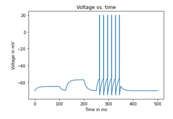
Figure 4.7: Output of sample code

Step 7: Explore your simulation
Now that you have designed an algorithm to plot Johnny’s experiment you are capable of learning a few characteristics of the design. For example, if you are curious about the voltage at a particular time step, you can read it out of the voltage vector. For instance, if you wanted to know the voltage at time point 2540 you would type:

print(voltageVector[2540])

If you wanted to change the strength of the applied stimulation, or the duration of each pulse, you may edit these lines:

stimVector[0:2000] = 0.5
stimVector[2500:4000]= 1.3
stimVector[5000:7000] = 2.0

Worked Example:
Johnny has now developed a general model of how a hippocampal neuron fires. But Mr. Firehydrant wants to know how both the length of the stimulation pulse and the strength of that pulse interact to influence the neuron’s firing. Johnny devises the following stimulation protocol:

At time zero, the cell is at rest. When the cell is not being stimulated, it is allowed to go back to rest.
At 0.5 ms, 5 nA of current is injected into the cell for one time step.
From 50 to 54 ms, 5 nA are injected into the cell.
At 150 ms, the applied current is turned back on at 15 nA for one time step.
From 200 ms to 202 ms, the current is held at 15 nA.
At 250 ms, there is a 30 nA pulse of injected current for one time step.
From 300 to 301 ms, the applied current is 30 nA.

This appears more difficult than it is, and much of what you did for the previous example will help here. Graph the cell’s voltage over time as well as the external current over time. Notice how increasing the duration of the current pulse provides an additive effect in bringing the cell’s membrane potential closer to threshold.

Most of your previous simulation can be recycled in full. You will make changes to two sections: defining your stimulation vector, and in adding a second graph. Here, we set the stimulation protocol.

# Begin by setting the default stimulation level to 0
stimVector = np.zeros(len(timeVector))

# At 0.5 ms, 0.5 nA of current is injected
stimVector[timeVector==0.5] = 5

# From 50 to 54 ms, 5 nA are injected into the cell
tStart = np.where(timeVector==50)[0]
tEnd = np.where(timeVector==54)[0]
stimVector[tStart[0]:tEnd[0]] = 5

# At 150 ms, 15 nA is injected for one time step
stimVector[timeVector==150] = 15

# From 200-202 ms, the current is held at 15 nA
tStart = np.where(timeVector==200)[0]
tEnd = np.where(timeVector==202)[0]
stimVector[tStart[0]:tEnd[0]] = 15

# A pulse of 30 nA at 250 ms
stimVector[timeVector==250] = 30

# From 300 to 301 ms, the applied current is 30 nA
tStart = np.where(timeVector==300)[0]
tEnd = np.where(timeVector==301)[0]
stimVector[tStart[0]:tEnd[0]] = 30

And this code snippet creates our two plots.

# This sets the plot object
plt.figure()

# This defines that we are plotting into the top plot
plt.subplot(2,1,1) # two rows, one column, first graph

# Plots time on the x-axis and current on the y-axis
plt.plot(timeVector, stimVector)

# Labels the x-axis
plt.xlabel('Time in ms')

# Labels the y-axis
plt.ylabel('External current in nA')

# Titles the plot
plt.title('External Stimulation vs Time')

# This defines that we are plotting into the top plot
plt.subplot(2,1,2) # 2 rows, 1 column, 2nd graph

# Plots time on the x-axis and voltage on the y-axis
plt.plot(timeVector, voltageVector)

# Labels the x-axis
plt.xlabel('Time in ms')

# Labels the y-axis
plt.ylabel('Membrane potential in mV')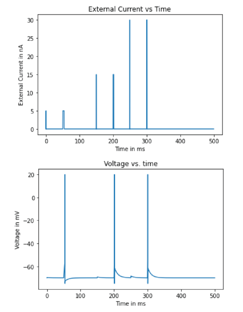

The plot looks like this:

Figure 4.8: Output of sample code

4.7 Summary

4.7.1 Passive membrane model:

The neuron is like a battery. We can assign different characteristics in a neuron to different parts of a circuit:
- Cell membrane = capacitor
- Ions = charge (Q)
- Current = injected stimulus (I)
- Voltage = membrane potential (V)
We can use concepts from Ohm’s law to model a neuron’s capacitance:
- \(Q = C_mV_m\)
We can use the GHK equation to compute the resting potential of a neuron.
- \(V_{m} = \frac{RT}{F}ln(\frac{P_{K}[K+]_{out}+P_{Na}[Na+]_{out}+P_{Cl}[Cl-]_{in}}{P_{K}[K+]_{in}+P_{Na}[Na+]_{in}+P_{Cl}[Cl-]_{out}})\)
We can combine the concepts listed above to model the change in voltage of a cell!
- For circuits in parallel, the currents will sum.
- \(\tau_m \frac{dV_m}{dt} = R_m I_e + E_L-V_m\)
Leaky integrate and fire:
- The leaky integrate and fire model is a way to model a neuron’s membrane potential using code.
  - In this model, current needs to be injected into the neuron, and as a result the neuron will produce a spike, which is modeled as an action potential.
  - It represents a neuron as a combination of conductance (the “leaky resistance”) and a capacitor.
- This model operates on the assumption that most stimuli give rise to roughly the same spike forms (i.e. that interspike intervals do not vary for a given stimulus).
- This model cannot store information regarding previous spike activity because it resets the membrane potential after each spike is fired.

4.7.2 An action potential has six phases:

Resting phase: when only the sodium-potassium pump and leakage channels are open.
The threshold: activation of voltage-gated sodium and potassium channels.
Depolarization: net increase in membrane potential as a result of the flow of sodium ions into the cell through the open voltage-gated sodium channels.
Overshoot: inactivation of sodium channels and activation of potassium channels.
Repolarization: net decrease in membrane potential back to its resting potential as a result of the flow of potassium ions out of the cell through the open voltage-gated potassium channels.
Hyperpolarization (undershoot): open voltage-gated potassium channels that cause the membrane potential to fall below the resting potential. An action that is corrected by the sodium-potassium pump and the leakage channels.

4.7.3 Main features of an action potential:

The sodium-potassium pump and leakage channels are ALWAYS functioning.
Potassium channels are slow to open and slow to close.
At resting membrane potential, the inside of the cell has a net negative charge and the extracellular contents are more net positive.
Ions will always follow both their electrical and concentration gradients unless some process prevents them from doing so.
The positive feedback loop causes depolarization and the negative feedback loop causes repolarization.

Figure 4.9: Example of an action potential.

4.7.4 The flow of ions and equilibrium potentials

The main idea: equilibrium potentials are dictated by the separation of charges and the distribution of ions across the membrane.
There are two types of equilibrium potentials that influence action potentials:
1. Membrane Potential: the electrical potential when the sum of all electrical concentration gradients of each species of the intracellular and extracellular ion at a specified time are at equilibrium.
2. Nernst Potential: the electrical potential when the force of the concentration gradient matches the electrical force attracting or repelling a specific species of ion.
  - Is also referred to as the reversal potential.
  - Each species of ion has its own Nernst potential.

4.8 Exercises

4.8.1 Conceptual Exercises

Describe the life cycle of an action potential. Be sure to include changes in channels/pumps, ion movement, and voltage.
Explain why the resting potential is a steady state and how ion permeability and Nernst potential play a role.
What does the Goldman-Hodgkin-Katz (GHK) equation tell you and when should it be used?
What are the different ways ions can move across the membrane of the neuron?
Water flow abides by similar rules as ions flowing across a membrane in a neuron. Match each aspect of ion flow to water flow below. Explain your reasoning.
Explain how depolarization and hyperpolarization relate to positive/negative feedback.

Figure 4.10: Match each part of the water flow in this dam to ion flow in a neuron.

Water Concept	Neural Concept
Water	Voltage-gated channel
Dam	Ions
Jet	Ion pump

Explain the basic function of the leaky integrate and fire model. Your response should describe both the RC membrane circuit as well as the logical rules governing the model neuron’s firing.
Describe one aspect of the leaky integrate and fire model that is not biologically realistic.
Briefly explain the concept of driving force.
Explain the difference between the membrane potential, Nernst potential and equilibrium potential.

4.8.2 Coding Exercises

Let us walk through calculating the Nernst potential in Python. 1. Shown below is the Nernst equation that allows us to calculate the Nernst potential (AKA: reversal potential, resting potential) of the crucial ions (Na+, K+, Cl-) in our body that make action potentials possible.
\[E_{ion} = \frac{RT}{zF}ln(\frac{[out]}{[in]}) \] Okay, I know this equation may seem to be made up of lots of different variables, but it really is not. Let’s break it down together:

R and F are both constants.
T is our body temperature.
So, \(\frac{RT}{F}\) is about 26.5 mV.
z is the charge of the given ion. (Hint: Na+: +1, K+: +1; Cl-: -1)
[out] and [in] refer to the ion concentrations on the extracellular, and intracellular sides of the membrane, respectively.

Our goal is to create a general Python function that will predict whether the Nernst potential for Na+, K+, or Cl- will be positive or negative. The advantage of writing a function is that we will be able to write one piece of code that can be re-used for each ion by substituting in the relevant values. Right now, we only care about the relative concentrations, so we can just use 1 to represent the side with the lower concentration, and 2 for the side with the higher ion concentration. Use the following steps to construct your function:

Open a blank Jupyter notebook.
Import the necessary Python libraries. (Hint: numpy is useful for calculation. In Python, ln() implemented in the log() function)
Set up the general function definition. (Hint: Use “def” and “return” to set up a function named “Eion” with three arguments. The constants in the Nernst equation will not affect our results, so we may omit them for now.)
Try out your function for each of the three major ions and print out the results. (Hint: Think about the relative concentration of each ion inside and outside of the neuron during the resting state. Remember that Cl- is tricky!)

Good job! Now, let’s apply your function to calculate more realistic Nernst potentials for Na+, K+, and Cl- given their actual ionic concentrations:

Ion	Intracellular concentration (mM)	Extracellular concentration (mM)
Na+	15	145
K+	150	4
Cl-	10	110

Pro-tip: We are still using the same Jupyter notebook as part (a), we do not have to import numpy again! Lazy is good.

Use the following steps to apply your function:

Set up the general function. (Hint: alter your Eion function to use the R and F constants as well.)
Use the values from the table in order to print out the Nernst potential for each ion.

Sort the Nernst potentials from smallest to largest. Print the name of the ion that is closest to the neuron’s resting potential (-65 mV).

As we previously learned, the resting potential of the neuron can be predicted by the Goldman Hodgkin Katz (GHK) equation as follows:
\[V_{m} = \frac{RT}{F}ln(\frac{P_{K}[K+]_{out}+P_{Na}[Na+]_{out}+P_{Cl}[Cl-]_{in}}{P_{K}[K+]_{in}+P_{Na}[Na+]_{in}+P_{Cl}[Cl-]_{out}}) \]
The first part of the equation looks similar to the Nernst equation - great!
\[V_{m} = 26.5 \cdot \ln(\frac{P_{K}[K+]_{out}+P_{Na}[Na+]_{out}+P_{Cl}[Cl-]_{in}}{P_{K}[K+]_{in}+P_{Na}[Na+]_{in}+P_{Cl}[Cl-]_{out}}) \]

But what the heck is going on inside the parentheses?

The resting potential is dependent on and made up of these three ions. Therefore, we are weighting each ion according to its relative permeability value. The relative permeability value reflects the ease with which each ion can pass through the membrane at rest. By convention, we assign \(P_{K+}\) to be 1. The membrane is far less permeable to sodium (\(P_{Na+} = 0.05\)), and moderately permeable to chloride (\(P_{Cl-} = 0.45\)). These values reflect the relative density of leak channels for K+, Na+, and Cl- in the membrane.

Create a general Python function to calculate the resting potential of a neuron from the previously provided values. Use the following steps:

Import the necessary Python libraries.
Set up the general function. There are six different concentrations that can be considered as input arguments. For simplicity, you may “hard code” the permeability of Na+ and K+ inside your function. Please put Cl- permeability as an argument to your function because you will use it in the next question. (Hint: take a close look at the equation. Cl- is different!)

Early in development (when we were babies), it is found that intracellular concentration of Cl- ions is higher than the extracellular concentration of Cl-. This is due to the delayed expression of Cl- exporters in the membrane. All else being equal, how would this affect the resting potential? Would the neuron be more or less likely to fire an action potential in this state?

To simplify, assume that \(p_{Cl} = 0.1\) because there are fewer exporters. Let’s assume that [ion] and [out] are switched for this problem.