Chapter 6 Firing Rates
6.1 Vocabulary
- Interspike interval (ISI)
- Integration window
- Time bin
- Spike train
- Spike count rate
- Coefficient of variation (CV)
- Fano factor
- Poisson process
- Homogeneous poisson process
- Inhomogeneous poisson process
6.2 Introduction
In the previous two chapters, we have seen manmade models that are built to represent the firing patterns of a neuron. What these models lack, however, is how the level of input changes over time. If we attempt to use the Hodgkin and Huxley model to represent a neuron, we would see a neuron with a constant firing rate, as observed in Figure 6.1 below.

Figure 6.1: An example of a simulated neuron using the Hodgkin Huxley equation.
If we compared this to an actual neuron’s firing rate, we would see something more similar to Figure 6.2.

Figure 6.2: Variability across four repetitions of the same stimulus. Figure taken from Gerstner et al, Neuronal Dynamics
As we can see, the most telling difference between the two graphs is that in our Hodgkin-Huxley model, the interspike interval, which is the distance between each spike, remains constant. In the measured activity of the real neuron, the interspike interval varies over time. In order to create a model that more accurately depicts the firing rate of a neuron, we need to be able to conceptually measure the firing rate of a neuron over time. In this chapter, we will discuss the three main approaches of measuring the firing rate of a neuron. Knowing how to measure firing rates will further our ability to create models of real neurons. By comparing measured firing rates with Poisson processes, we can model the variability of interspike intervals in real neurons.
6.3 Spike Trains
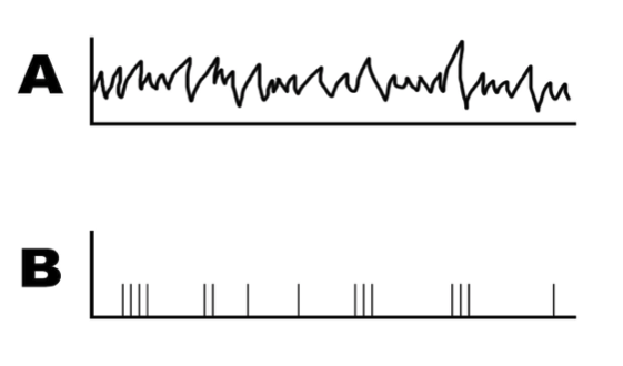
Figure 6.3: Example of a spike train. Graph A shows the recorded stimulus and graph B shows the recorded actions potentials during the stimulus.
Assume that we measured a neuron firing in response to a random sensory stimulus (shown in Figure 6.3a), and we recorded its voltage changes and displayed the signal in an oscilloscope. How should we analyze the information encoded in these action potentials?
As we’ve previously discussed, action potentials are an all-or-none event. This characteristic allows us to represent spikes in a binary fashion. To do this, we need to remember that the axes of both graph A and B represent voltage over time. When the voltage surpasses the threshold, a spike occurs. The length of time over which the neuron is recorded is called the integration window: we will first break up this window into lengths of time small enough that they can only contain one spike. This small increment of time is called a time bin. With this in mind, a voltage response curve can be reduced to time-bins that either contain a spike (represented in a binary fashion by a 1) or do not (represented by a 0). This time-dependent sequence of 1s and 0s is referred to as a spike train, depicted in graph Figure 6.3b.
Another characteristic of action potentials is that they are stereotyped: they are consistent with each other in voltage. This means that when neurons communicate with each other, the peak voltage never changes - all the information must be conveyed in the rate or timing of the action potentials. Although we’ve reduced the response of our neuron down to a train of 1s and 0s, we have the information we need to analyze what caused the original neuron to fire. Before being able to analyze the data in these spike trains however, we need to figure out how we plan to represent them.
Practice Problem 1: For this example, we will consider data collected by Robert Cat from a neuron located in an alien’s posterior inferior temporal cortex responding to a rapidly-changing color stimulus. Dr. Cat recorded the neuron at 1000 Hz for ten seconds and created a Boolean vector (spike train) where 1 signifies a spike. Create a program that calculates the neuron’s spike count rate, and then create a plot of the spike count rate versus time.
# First, import the necessary libraries
import numpy as np
import matplotlib.pyplot as plt

# Calculate the total number of spikes and store them in totalSpikes
# Because the vector is binary, the sum of the 1s and 0s gives the total
totalSpikes = np.sum(spikes)

# Calculate the neuron’s spike count rate, and store it in spikeRate
# We divide by 10 because we want our rate to be in the unit of spikes/second (Hz)
spikeRate = totalSpikes / 10

# Print the spike count rate
print('The spike count rate is: {} Hz'.format(spikeRate))
6.4 Spike Statistics
There are multiple ways to go about representing the spike train data from Figure 6.3B, each with its advantages and disadvantages. Firstly, we can find the spike count rate , a measurement of the number of spikes over our length of time. This returns a number expressed in spikes/second, or Hz. The simplicity of this approach allows for easy application of our firing rate to mathematical models such as neural networks. For example, one can take a spike count rate and use it in a Poisson process, , an idea we’ll discuss later. However, the problem with this approach lies in the fact that given our output, we don’t know how the spikes are distributed temporally. In Figure 6.3B, some sections of the graph have dense areas of spikes, while others have longer periods without spikes. Recreating our spike train with this method would eliminate this temporal information. Because of the same principle, this model also fails to capture changes in neuronal activity that might occur when the stimulus is changed during our period of measurement.
In vitro, the timing of neural responses are highly variable and the response of a neuron to the same stimulus may even vary from trial to trial (Mainen & Sejnowski, 1995). To account for cross-trial variability, we can also analyze results from multiple trials to get a better estimate of the average neural response. This provides us with our second method of analysis: spike density. Here, we measure the same neuron over multiple trials of the same length to determine the reliability of spike times. This allows us to maintain the temporal information that our previous method of analysis eliminates. However, neuronal habituation can interfere with repeated trials; when a neuron is exposed to the same stimulus over and over again, neuronal activity typically decreases. One potential solution to this problem is mixing in randomly distributed stimuli into our trials. This method is also difficult to execute in a lab setting, as it can be difficult to keep a neuron around long enough to measure it multiple times.
Up until now, we’ve been discussing recordings from single neurons. Another method of analyzing neuronal activity is to instead record from a population of neurons that respond to similar stimuli. We refer to this method of analysis as population density. In the lab, this is accomplished by electrode arrays that measure each neuron’s response independently, and sampled over one trial. We can then average the activity of these neurons to get a sense of population-wide trends. Here, our output won’t contain information from individual neurons, and it requires that we assume the neurons we record from are all doing the same thing. However, it has biological plausibility in that it might mimic what a postsynaptic neuron “sees”: neurons receive signals from many inputs in vivo. Additionally, since we’re averaging over a population rather than over time, our output also contains the temporal information that the spike count rate does not include. However, this method is also difficult to execute in a lab - tools for multi-neuron recording are relatively recent advancements in the field of neuroscience. Table 6.1 notes the advantages and disadvantages to using each method of computing neuronal firing rate.
| Method | Definition | Advantages | Disadvantages | |
|---|---|---|---|---|
| Spike count rate | spikes/time of a single neuron, measured in Hz | (1) Easier than recording fill population; (2) Easy to use in case of building neural networks | (1) Temporal distribution of spikes is unclear; (2) Only works with unchanging stimulus or slowly changing stimulus | |
| Spike density | Firing rate of one neuron over multiple trials; time bins are used to obtain temporal information | (1) Temporal distribution is available; (2) Reliable over trials | (1) Neuron may be sensitized after repeated stimulation (habituation); (2) Lack of generalization – you’re finding one neuron’s preference | |
| Population density | Records spike trains of multiple neurons over the same trials | Shows us population-wide trends | (1) Difficult to record from multiple neurons simultaneously; (2) Assumes all neurons are the same |
Here is a way of seeing the same information visually:
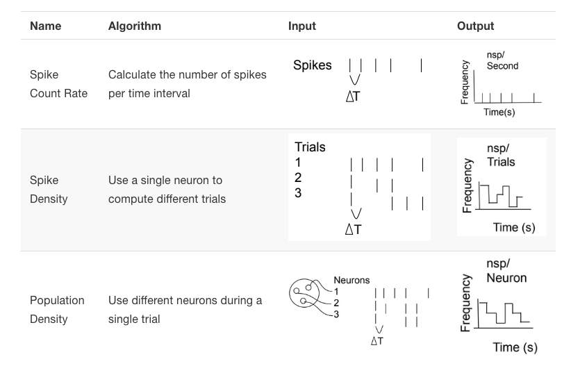
Figure 6.4: Comparing the three methods for computing firing rate
Peristimulus time histograms (PSTHs) can be used to describe spike trains. These plots are created by dividing our period of measurement into time periods of some established length, and graphing the number of spikes in each of these periods over time. These are typically lined up temporally with a graph of stimulus intensity in order to visualize how neuronal activity is correlated to the stimulus. These are useful tools in our arsenal to analyze spike trains.
Sometimes, instead of collating data from real neurons, we need to simulate spike trains from given statistics. These artificial spike trains can be compared with real data, or used to reconstruct possible firing patterns with a given stimulus. Here, we will discuss Poisson processes, a tool we can use to generate artificial spike trains.
Worked Example:
Next, we will examine how to calculate the rate as an average across 50 trials of the same neuron Dr. Cat obtained responding to the same stimulus using the spike density rate. In this experiment, each trial was one second long, and measurements were taken at 1000 Hz. Dr. Cat noticed in their research that the neuron fired at an average of 50 Hz for the first 300 ms of the recording and an average of 15 Hz for the remaining 700 ms. First, simulate the neuron in Dr. Cat’s experiment and then, using this information, plot spike density rate versus time.
# As usual, we'll begin by importing the necessary libraries
import numpy as np
import matplotlib.pyplot as plt

# Define the two average spiking rates as probabilities
p1 = 50/1000 # on average, 50 spikes in the 1000 time points
p2 = 15/1000 # on average, 15 spikes in the 1000 time points

# In order to create the data, we will create a matrix that
# is numTrials by numTimePoints in size. We will initialize
# it with zeros and then fill in the spikes later.
dataMat = np.zeros((50, 1000))

# Here, we will create a nested loop. The outer loop will
# loop through the 50 trials. The inner loop will loop through
# the time points and use a random number generator to determine
# the placement of each spike.

# Data creation loop of 50 trials
for j in range(50):

  # In each of the 50 trials, loop through 1000 time points
  for i in range(1000):

    # At each time point, we want the neuron to fire with
    # probability p1 in the first 300 ms, and probability p2
    # for the remainder of the trial.

    # To do this, we will first create a conditional to determine
    # whether or not we are in the first 300 ms. If so, we will
    # use p1, and if not, we will use p2.
    if i < 300:
      p = p1
    else:
      p = p2

    # At each time point, we flip a random coin using np.random.rand().
    # This generates a random value between 0 and 1. If this value
    # is less than our target probability, the neuron will fire.
    if np.random.rand() < p:
      dataMat[j, i] = 1

    # Note that we do not need an "else" here because the rest of the
    # matrix is already 0.

# Now that we have created our data, we can calculate the spike
# density rate.

# Sum all the trials to plot the total number of spikes in each
# time bin, and store them in counts (HINT: we wish to sum over
# all the rows, and numpy denotes rows before columns. This is
# the reason we use axis=0 (i.e. the first axis))
counts = np.sum(dataMat, axis = 0)

# Now, we need to translate these counts into a rate by dividing
# by the number of trials and the dt
density = (1/(1/1000)) * counts/50

# In order to create a plot, we need to create a vector of time
# points to plot it against
time = np.arange(1000)

# Create spike density vs. time graph
plt.figure()
plt.plot(time, density)
plt.xlabel('Time in ms')
plt.ylabel('Spike density (Spikes per second)')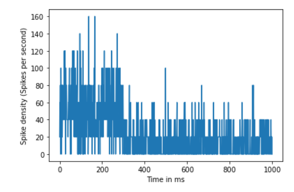
Figure 6.5: Spike density rate over 50 trials
6.5 Poisson Processes
Before we can talk about Poisson processes, let’s establish some mathematical definitions. A Fano factor is found by dividing the variance of the interspike intervals (time between each spike) over a dataset over the mean interspike interval of the data. We do this to see if the distribution of the data (in our case, spikes) is random in our period of measurement.
\[F = \frac{\sigma_{sp}^2}{\mu_{sp}}\]
The ISI histogram can be characterized by coefficient of variation (CV), which is the standard deviation of ISIs divided by the mean of it. Apart from that, we can also use the Fano factor to measure the spike variability. It is calculated by the variance of the number of spikes divided by the mean number of spikes in a given time interval. Compare to CV, Fano factor is less dependent on the intervals between spikes but more on the number of spikes in a given time bin. If the underlying firing rate varies or the spike firing in irregular time points, both CV and Fano factor increase. Thus, CV and Fano factors are useful secondary statistics that helps to measure variability in spike trains.
A Poisson process is a dataset that, when analyzed like this, returns a Fano factor of 1, meaning that the variance and the mean are equal. This means that in our time period, the probability of a spike occurring at each time interval is equal to the number of spikes that occur over the time interval. To understand this abstract definition, think about a timeline of 100 seconds where one time point is equal to one second along the timeline. We know that at 50 time points along the timeline, we get a value of 1. From this information, we know that the probability of a 1 occurring is 50/100 (occurrences/length of time) at each time point. So, for each time point, we flip a coin. When it’s heads, we record a 1. When it is tails, we record a 0. We agree that all 1s will be randomly spread along the timeline, and the interval between when we get a pair of heads varies along the timeline. This will look very similar to an artificial spike train generated by the Poisson process, whose distribution can be expressed by the formula below.
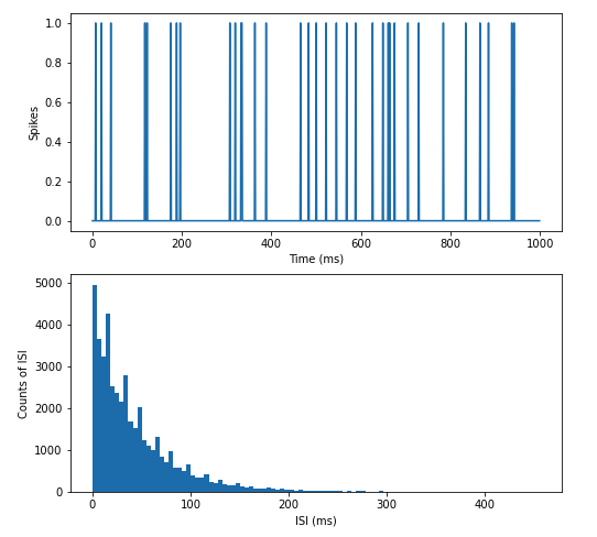
Figure 6.6: An artificial spike train generated by Poisson process and its ISI distribution. Notice that the spikes are randomly distributed along the time axis, and the ISI histogram has an exponential distribution.
Thus, the formula for the probability of q spikes in some small interval \(\Delta t\) is:
\[p(q\ spikes\ in\ \Delta{t}) = e^{-\lambda}\frac{\lambda^{n}}{n!} \]
What makes this Poisson process homogeneous is that our known firing rate (for this example, 45 Hz) does not change over our 1000 ms time period. This means that for every millisecond in this period, there is a 45/1000 chance to find a spike there.
By contrast, an inhomogeneous Poisson process is one in which our firing rate changes sometime during our time period. For example, we could establish that starting at 500 ms, our firing rate would increase to 65 Hz. This would mean for every subsequent millisecond, there would be a 65/1000 chance to find a spike there.
Creating a distribution of the ISIs from a spike train allows us to compare it to a Poisson process. In a fully random distribution of spikes, one would expect to find an exponential distribution of interspike intervals decreasing in length. This is shown in Figure 6.6 which depicts a histogram of ISIs from a homogeneous process. It is evident that most ISIs are small, with some very long ISIs.
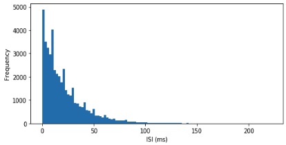
Figure 6.7: Distribution of ISIs from a randomly firing artificial neuron.
Worked Example Below is a section of code that will allow you to create a digital neuron that fires based on a Poisson process. This model can help aid our understanding so that we can create more biologically plausible ones as we grow to be more mature hackers.
Some metrics to keep in mind as we go through this code block:
- This neuron fires at a constant rate of 15 Hz, but at random intervals.
- The simulator samples 1000 times a second (1000 Hz).
- The simulator runs for 2 minutes.
- We will compute the spike count rate for this neuron and plot the distribution of interspike intervals as well.
# Import necessary libraries
import numpy as np
import matplotlib.pyplot as plt

# Define the probability of a spike occurring in each interval
prob = 15/1000
# We are sampling 1000 times/s and the neuron fires 15x/s on average

# Initiate data structure to hold the spike train
timePoints = 2 * 60 * 1000 # 2 minutes * 60s/minute * 1000 samples/second
poissonNeuron = np.zeros(timePoints)

# Create a loop to simulate each time point
for i in range(len(poissonNeuron)):
  # conditional statement to asssess if spike has occurred
  if np.random.rand() < prob: # if a random number between 0 and 1 is < prob
    # store a 1 in poissonNeuron. This means the neuron has fired
    poissonNeuron[i] = 1

# Compute the overall spike count rate
numSpikes = sum(poissonNeuron)
# total number of action potentials in 2 minutes
print('The spike count rate was {} Hz'.format(numSpikes / 2*60))
# 2 minutes * 60s/minute

# Plot the distribution of ISIs
# Step 1: determine the time stamps of each spike
spikeTimes = np.where(poissonNeuron == 1)[0]
# Remember the difference between = and ==
# The [0] at the end is because np.where returns two arrays and we
# only need the first one

# Step 2: Initialize data structure to hold ISIs
isi = np.zeros(len(spikeTimes)-1)
# There will be one fewer ISI than the number of spikes

# Step 3: Loop through each pair of consecutive spikes, compute isi
# and store
for x in range(len(isi)):
  # Each ISI is the time between spike x and spike x+1
  isi[x] = spikeTimes[x+1] - spikeTimes[x]

# Plot the ISI distribution
plt.hist(isi, 110) # create a histogram with 110 bins
plt.xlabel('ISI (ms)')
plt.ylabel('Frequency')
6.6 Summary
Translating neuronal activity to a format where it can be used in mathematical operations makes use of the fact that action potentials (spikes) are all-or-none and stereotyped. Because of this, every spike both occurs at the same threshold and consistently follows the same pattern. By representing spikes and their absence in a binary system, we can create spike trains that distill voltage activity into vectors of 1s and 0s.
In many applications, estimating the continuous firing rate of a neuron is advantageous. There are multiple approaches to doing so. The three major methods are:
- Spike count rate
- Spike density
- Population density
We then turn to the Poisson process, which is a tool for generating artificial spike trains when the firing rate over a time period is known. These artificial spike trains create a random distribution of spikes by dividing the known firing rate by the time period. This gives us a probability that a spike will occur at each time point. Because the fact that a spike will/will not occur is random at each time point (like flipping a coin), we create the random distribution of spikes. We can compare real neuronal spike trains with spike trains generated by Poisson processes to learn more about possible neuronal responses to stimuli.
6.7 Exercises
6.7.1 Conceptual Problems
Define the spike count rate. What are the advantages and disadvantages of defining rate as a spike count?
Define the spike density rate. What are the advantages and disadvantages of defining rate as a spike density?
Define firing rates as population density. What are the advantages and disadvantages of defining rate as population activity?
What are the qualifications for a Poisson spike train?
Challenge: We have simulated a homogeneous Poisson process. What would you alter in this code in order to simulate an inhomogeneous Poisson process?
6.7.2 Coding Problems
- Part a. Create a Poisson spike train to simulate a neuron that fires for 2000 ms at an average rate of 50 Hz. The Poisson distribution is a useful concept to create random spike locations within a time frame (2000 ms in this case) that produce an average desired frequency (50 Hz in this case). The randomness can be achieved by using the np.random.rand() function, which generates a random value uniformly sampled between 0 and 1. If this random value is less than the specified probability of firing, than the code will generate a 1 indicating a spike. Otherwise, the spike train will contain zeros.
Part b Using the following code template, add a counting variable to measure the number of spikes produced in the simulation. Use this total spike count to calculate the final spike count rate (spikes/second, or Hz) and see how it compares to the desired frequency of 50 Hz (50 spikes/second).
# Import the necessary libraries
import matplotlib.pyplot as plt
import numpy as np

# Initialize data structures
# Hint: your simulation runs for 2000 ms
timeVec =

# Hint: you may express your desired rate as a nSpikes / 1000 ms probability
probability =

# Hint: you want the default value to be zero
spikes =

# Loop through each time point - fill in missing code
for i in range():
  if np.random.rand() < probability:
    # fill in this key line

# Compute the spike count rate here
spikeCountRate =

# Print the spike count rate
print('The firing rate was: {} Hz'.format(spikeCountRate))

# Create a figure of the spike train
plt.figure()
plt.plot(timeVec, spikes)
plt.title('Spikes versus Time')
plt.xlabel('Time (ms)')
plt.ylabel('Spikes')
Part c Using your spike train, compute a histogram of interspike intervals (ISIs). To do this, it will be helpful to find the locations of your spikes in your spike train. The function np.where() will do this (hint: you will only need the first value returned in the tuple). Hint: you will have 1 fewer ISI than number of spikes in your spike train.
- Part a Using the same Poisson process as above, simulate an experiment in which 40 trials of 2000 ms are created and place all trials into a single array. Fill in the code snippet below to create your array and plot a raster plot of all trials.
# Import necessary libraries
import numpy as np
import matplotlib.pyplot as plt

#fill in the time vector and the spike frequency value of 50 Hz
timeVec =
p1 =

#Allocate space for the 40 trials x 2000 ms array
allTrials =

#Create a Poisson spike generator, that loops 40 times for all 40 trials
for i in range():

    # For each trial, use an inner loop to represent all 2000 time points
    for v in range():

# Create the raster plot
for j in range(): # How many trials are we running?
    spikes, =  #Fill in Spikes to represent every spike found
               # in the allTrials matrix. Index the jth trial
               # only.

    spikeTimes = timeVec[spikes]
    theseSpikes = np.ones(len(spikes))*j+1

    plt.scatter(spikeTimes, theseSpikes, s=2, c='k')

#Fill in the labels of the x, y axis
plt.title()
plt.xlabel()
plt.ylabel()
Part b Now compute the Fano factor for your spike array. This may be done in one line of code using the built-in functions for variance and mean from the numpy library.